Introduction
The bgms package implements Bayesian methods for analyzing graphical models. It supports three variable types:
- ordinal (including binary) — Markov random field (MRF) models,
- Blume–Capel — ordinal MRF with a reference category,
- continuous — Gaussian graphical models (GGM).
The package estimates main effects and pairwise interactions, with optional Bayesian edge selection via spike-and-slab priors. It provides two main entry points:
-
bgm()for one-sample designs (single network), -
bgmCompare()for independent-sample designs (group comparisons).
This vignette walks through the basic workflow for ordinal data. For
continuous data, set variable_type = "continuous" in
bgm() to fit a Gaussian graphical model.
Wenchuan dataset
The dataset Wenchuan contains responses from survivors
of the 2008 Wenchuan earthquake on posttraumatic stress items. Here, we
analyze a subset of the first five items as a demonstration.
Fitting a model
The main entry point is bgm() for single-group models
and bgmCompare() for multiple-group comparisons.
fit = bgm(data, seed = 1234)Posterior summaries
summary(fit)
#> Posterior summaries from Bayesian estimation:
#>
#> Category thresholds:
#>                 mean  mcse    sd    n_eff  Rhat
#> intrusion (1)  0.475 0.007 0.240 1029.573 1.002
#> intrusion (2) -1.904 0.013 0.341  700.335 1.003
#> intrusion (3) -4.851 0.022 0.556  646.071 1.005
#> intrusion (4) -9.522 0.034 0.891  702.595 1.006
#> dreams (1)    -0.595 0.006 0.198  976.982 1.002
#> dreams (2)    -3.803 0.012 0.361  915.211 1.001
#> ... (use `summary(fit)$main` to see full output)
#>
#> Pairwise interactions:
#>                    mean  mcse    sd    n_eff n_eff_mixt  Rhat
#> intrusion-dreams  0.315 0.001 0.034 1292.695            1.003
#> intrusion-flash   0.169 0.001 0.032 1338.535            1.001
#> intrusion-upset   0.099 0.002 0.033  265.807    219.571 1.038
#> intrusion-physior 0.098 0.005 0.035  458.654     57.357 1.076
#> dreams-flash      0.251 0.001 0.031 1424.804            1.005
#> dreams-upset      0.114 0.001 0.028  885.776    880.558 1.005
#> ... (use `summary(fit)$pairwise` to see full output)
#> Note: NA values are suppressed in the print table. They occur here when an
#> indicator was zero across all iterations, so mcse/n_eff/n_eff_mixt/Rhat are undefined;
#> `summary(fit)$pairwise` still contains the NA values.
#>
#> Inclusion probabilities:
#>                    mean  mcse    sd n0->0 n0->1 n1->0 n1->1 n_eff_mixt
#> intrusion-dreams  1.000       0.000     0     0     0  1999
#> intrusion-flash   1.000       0.000     0     0     0  1999
#> intrusion-upset   0.969 0.019 0.175    58     5     5  1931     85.449
#> intrusion-physior 0.953 0.045 0.212    92     2     2  1903
#> dreams-flash      1.000       0.000     0     0     0  1999
#> dreams-upset      0.999 0.001 0.032     1     1     1  1996
#>                    Rhat
#> intrusion-dreams
#> intrusion-flash
#> intrusion-upset   1.282
#> intrusion-physior 1.344
#> dreams-flash
#> dreams-upset      1.291
#> ... (use `summary(fit)$indicator` to see full output)
#> Note: NA values are suppressed in the print table. They occur when an indicator
#> was constant or had fewer than 5 transitions, so n_eff_mixt is unreliable;
#> `summary(fit)$indicator` still contains all computed values.
#>
#> Use `summary(fit)$<component>` to access full results.
#> Use `extract_log_odds(fit)` for log odds ratios.
#> See the `easybgm` package for other summary and plotting tools.
You can also access posterior means or inclusion probabilities directly:
coef(fit)
#> $main
#> cat (1) cat (2) cat (3) cat (4)
#> intrusion 0.4748091 -1.903948 -4.851133 -9.522112
#> dreams -0.5947650 -3.802846 -7.132969 -11.570727
#> flash -0.1131397 -2.575138 -5.393752 -9.705429
#> upset 0.4080633 -1.324809 -3.398199 -7.082666
#> physior -0.6159404 -3.164050 -6.211629 -10.555308
#>
#> $pairwise
#> intrusion dreams flash upset physior
#> intrusion 0.00000000 0.314546956 0.169225721 0.099074309 0.097572257
#> dreams 0.31454696 0.000000000 0.250679559 0.114415461 0.003597214
#> flash 0.16922572 0.250679559 0.000000000 0.003919395 0.154130991
#> upset 0.09907431 0.114415461 0.003919395 0.000000000 0.354342035
#> physior 0.09757226 0.003597214 0.154130991 0.354342035 0.000000000
#>
#> $indicator
#> intrusion dreams flash upset physior
#> intrusion 0.0000 1.000 1.0000 0.9685 0.953
#> dreams 1.0000 0.000 1.0000 0.9990 0.078
#> flash 1.0000 1.000 0.0000 0.0845 1.000
#> upset 0.9685 0.999 0.0845 0.0000 1.000
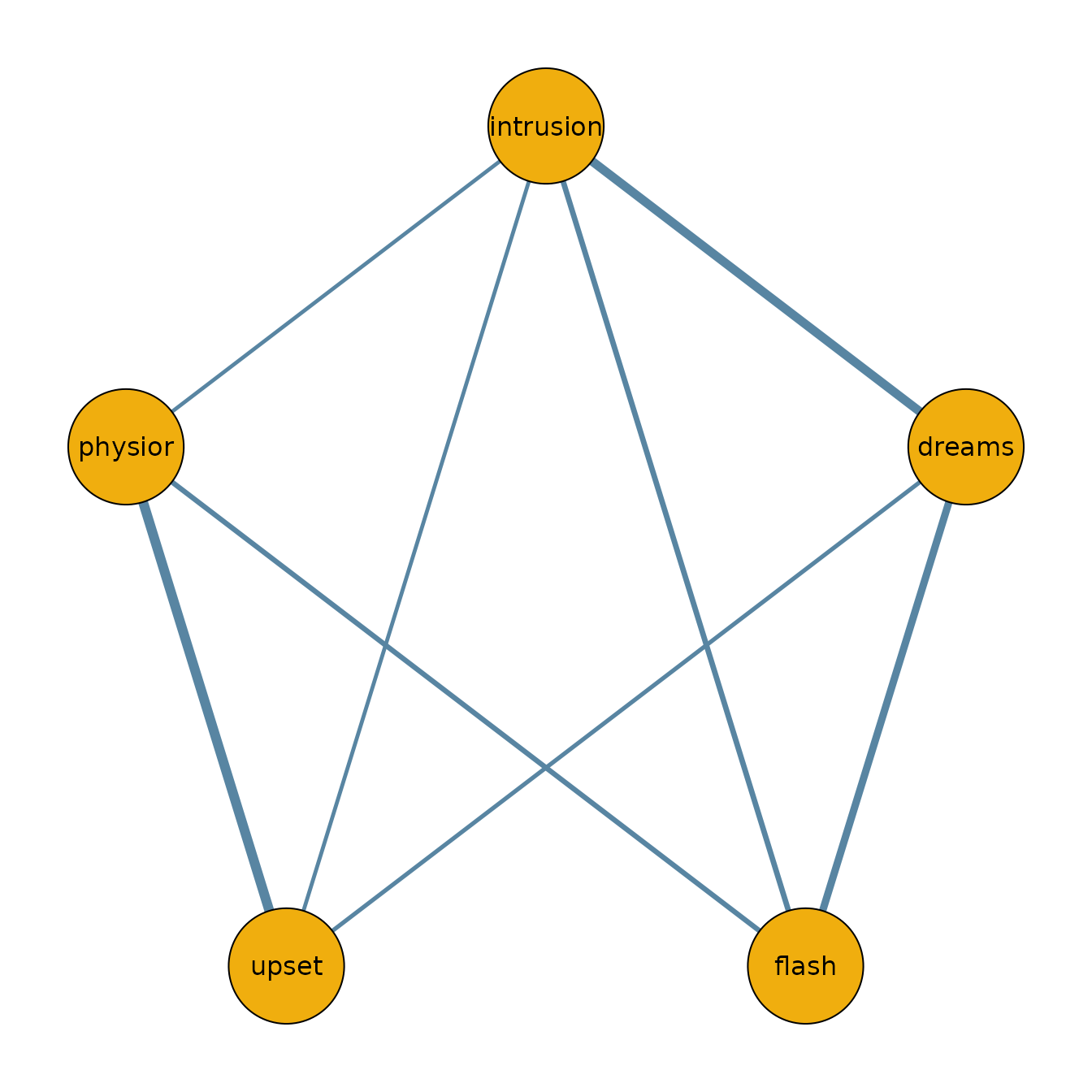
#> physior 0.9530 0.078 1.0000 1.0000 0.000Network plot
To visualize the network structure, we threshold the posterior inclusion probabilities at 0.5 and plot the resulting adjacency matrix.
library(qgraph)

median_probability_network = coef(fit)$pairwise
median_probability_network[coef(fit)$indicator < 0.5] = 0.0

qgraph(median_probability_network,
  theme = "TeamFortress",
  maximum = 1,
  fade = FALSE,
  color = c("#f0ae0e"), vsize = 10, repulsion = .9,
  label.cex = 1, label.scale = "FALSE",
  labels = colnames(data)
)
Continuous data (GGM)
For continuous variables, bgm() fits a Gaussian
graphical model when variable_type = "continuous". The
workflow is the same:
The pairwise effects are partial correlations (off-diagonal entries
of the standardized precision matrix). Missing values can be imputed
during sampling with na_action = "impute".
Next steps
- For comparing groups, see
?bgmCompareor the Model Comparison vignette. - For diagnostics and convergence checks, see the Diagnostics vignette.